01Control Design

Faster Response, Zero Steady-State Error

Root-Locus PD/PID Design and MATLAB Tuning

Control SystemsDecember 2025

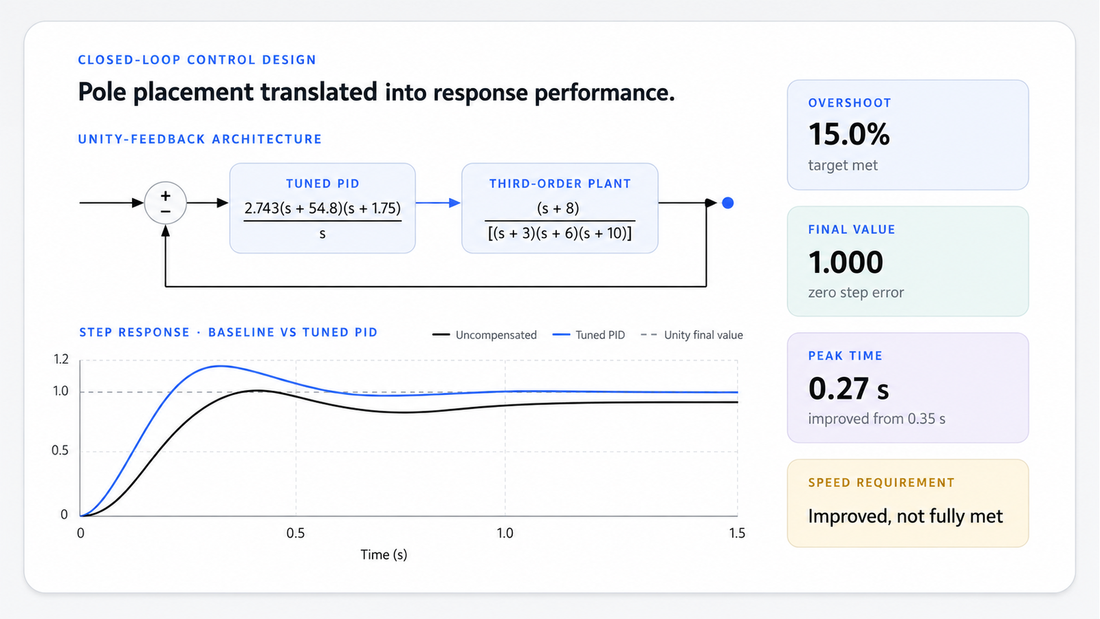
Starting from a third-order unity-feedback plant, this study used root-locus geometry to move the dominant poles toward a faster region of the s-plane, then added integral action and tuned the controller in MATLAB. The final PID response reached unity with 15.0% overshoot and a 0.27 s peak time—faster than the 0.35 s baseline, though still above the approximately 0.235 s design target.

Unity-feedback control loop with a tuned PID controller, a baseline-versus-tuned step-response chart, and final metrics of 15 percent overshoot, unity final value, and 0.27 second peak time. — Root-locus design and MATLAB tuning produced a faster unity-final-value response with 15.0% overshoot; the exact two-thirds peak-time target remained partially unmet.

02Context

Project Overview

The project treats a fixed third-order plant as a controller-design problem. The uncompensated system could be placed near the required damping ratio, but its response remained slower than desired and settled below unity for a step input.

The design progressed from an uncompensated baseline to PD compensation, then to a PID structure with integral action. Root-locus geometry established rational controller locations, while MATLAB step responses exposed the difference between dominant-pole predictions and the full higher-order closed loop.

The result is a complete analytical and simulation-based design study. It does not include a physical controller, real-time deployment, or laboratory measurements.

03Definition

Engineering Problem & Requirements

For the unity-feedback plant P(s) = (s + 8) / [(s + 3)(s + 6)(s + 10)], the control challenge was to maintain approximately 15% overshoot, reduce peak time to two-thirds of the uncompensated prediction, and eliminate step steady-state error.

The overshoot requirement corresponds to a damping ratio of approximately ζ = 0.517. The uncompensated dominant-pole design predicts T_p1 ≈ 0.352 s, giving a required target of T_p2 ≈ 0.235 s.

01Establish the uncompensated closed-loop baseline.
02Calculate the damping ratio associated with 15% overshoot.
03Determine the desired faster dominant-pole location.
04Use the root-locus angle condition to place a PD zero.
05Add integral action for zero step steady-state error.
06Compare dominant-pole predictions with complete MATLAB step responses.
07Tune the controller when the initial PID response does not match the overshoot target.
08Evaluate the final controller against every original requirement.

04Architecture

How the Closed Loop Is Shaped

A unity-feedback loop compares the reference with the output and passes the resulting error through the controller. The controller changes the open-loop pole-zero geometry; the plant itself remains unchanged.

01Reference input

02Tracking error

03Controller

04Third-order plant

05Closed-loop output

06Unity feedback

07Evaluate response

The PD term contributes phase and moves the root locus toward a faster region. The integrator increases the system type and removes step steady-state error.

Because integral action also adds a pole, the final transient response must be checked using the complete closed-loop model rather than assumed from the dominant pair alone.

Unity-feedback block diagram with reference input, summing junction, tuned PID controller, third-order plant, output, and feedback path. — The controller changes the open-loop pole-zero geometry while the third-order plant remains fixed inside a unity-feedback loop.

05Configuration

Design Stages & Parameters

The design preserves the plant and progressively changes the controller structure, gain, and zero locations. Reported dominant poles are analytical design values; step final values come from the complete MATLAB closed-loop responses.

Gain K

Uncompensated: 89.118
PD: 4.118
Initial PID: 2.9197
Tuned PID: 2.743

PD zero

Uncompensated: —
PD: −46.43
Initial PID: −46.43
Tuned PID: −54.8

PI zero

Uncompensated: —
PD: —
Initial PID: −1.5
Tuned PID: −1.75

Pole at origin

Uncompensated: No
PD: No
Initial PID: Yes
Tuned PID: Yes

Reported dominant poles

Uncompensated: −5.384 ± j8.916
PD: −7.494 ± j12.414
Initial PID: −6.1485 ± j10.1817
Tuned PID: Not reported

Step final value

Uncompensated: 0.798
PD: 0.895 before tuning
Initial PID: 1.000
Tuned PID: 1.000

Controller design stages and parameters
Parameter	Uncompensated	PD	Initial PID	Tuned PID
Gain K	89.118	4.118	2.9197	2.743
PD zero	—	−46.43	−46.43	−54.8
PI zero	—	—	−1.5	−1.75
Pole at origin	No	No	Yes	Yes
Reported dominant poles	−5.384 ± j8.916	−7.494 ± j12.414	−6.1485 ± j10.1817	Not reported
Step final value	0.798	0.895 before tuning	1.000	1.000

The plant transfer function remains unchanged through every stage.
The initial PID combines the root-locus-derived PD zero with a PI zero near the origin.
Final tuning changes both controller zeros and the gain.
These are continuous-time MATLAB model parameters, not deployed digital-controller constants.

S-plane plot showing the uncompensated dominant poles, desired compensated poles, PD-compensated poles, and initial PID dominant poles along the 0.517 damping-ratio direction. — Dominant-pole movement documents the analytical progression from the baseline toward a faster root-locus region before integral action modifies the final dynamics.

06Reasoning

Key Engineering Decisions

Six decisions connect the transient-response requirements to the analytical controller structure and the final MATLAB tuning.

Decision

Preserve the 15% damping-ratio line

Keep ζ ≈ 0.517 while defining the faster pole target.

Rationale: This separates the speed objective from the overshoot objective.
Trade-off: A constant damping ratio does not guarantee exactly 15% overshoot in the complete higher-order response.

Decision

Convert speed into a pole target

Set the desired peak time to two-thirds of the uncompensated prediction.

Rationale: Peak time gives a direct relationship to the desired imaginary pole component.
Trade-off: The dominant-pole approximation is only an initial design model.

Decision

Add one real PD zero

Use the root-locus angle condition to place a zero at approximately −46.43.

Rationale: The added phase allows the locus to pass near the faster desired region.
Trade-off: PD compensation improves transient speed but does not change system type or eliminate step error.

Decision

Place the PI zero near the origin

Add (s + 1.5) / s after the initial PD design.

Rationale: The integrator removes step steady-state error, while the nearby zero limits disturbance to the transient geometry.
Trade-off: The added pole weakens the second-order approximation and changes the overshoot.

Decision

Treat analytical design as the starting point

Verify every design stage with the full MATLAB closed-loop response.

Rationale: The initial PID reached unity but produced only 10.3% overshoot.
Trade-off: Additional tuning moves the final controller away from the first root-locus values.

Decision

Tune gains and zero locations together

Move the PD zero to −54.8, the PI zero to −1.75, and reduce the gains.

Rationale: These changes restore PID overshoot to 15.0% while keeping the final value at unity.
Trade-off: The final peak time improves but remains above the exact two-thirds target.

07Model

Root-Locus Mathematical Design

Damping-ratio, peak-time, and root-locus angle relations convert the response specifications into an analytical controller starting point.

Overshoot to damping ratio

ζ = −ln(OS) / √(π² + ln²(OS))

Maps the 15% overshoot requirement to ζ ≈ 0.517.

Peak time

T_p = π / ω_d

Relates the dominant-pole imaginary component to predicted peak time.

Faster target

T_p2 = (2 / 3)T_p1

Sets the required peak time to approximately 0.235 s.

Desired dominant pole

s_d ≈ −7.82 ± j13.37

Combines the selected damping ratio with the faster peak-time target.

Root-locus angle condition

Σ∠(s_d − z_i) − Σ∠(s_d − p_i) = (2k + 1)180°

Determines the additional controller phase required at the target pole.

Required PD phase

φ_c ≈ 19.1°

Represents the calculated phase deficit at the desired location.

PD-zero location

z_c = |σ₂| + ω_d2 / tan(φ_c) ≈ 46.43

Places the added real zero at approximately s = −46.43.

Initial PID

C_initial(s) = 2.9197(s + 46.43)(s + 1.5) / s

Adds integral action to the root-locus-derived PD structure.

Tuned PID

C_tuned(s) = 2.743(s + 54.8)(s + 1.75) / s

Records the final MATLAB-tuned controller used for response evaluation.

Required overshoot

Value: 15%

Damping ratio

Value: 0.517

Uncompensated predicted peak time

Value: 0.352 s

Required peak time

Value: 0.235 s

Desired dominant pole

Value: −7.82 ± j13.37

Root-locus phase deficit

Value: 19.1°

Initial PD zero

Value: −46.43

Root-locus design quantities
Design quantity	Value
Required overshoot	15%
Damping ratio	0.517
Uncompensated predicted peak time	0.352 s
Required peak time	0.235 s
Desired dominant pole	−7.82 ± j13.37
Root-locus phase deficit	19.1°
Initial PD zero	−46.43

The root-locus calculation is a dominant-pole design method. It provides a defensible starting controller but does not replace evaluation of the complete third- and fourth-order closed-loop systems.

The distinction matters most after integral action is added. The initial PID dominant pair suggests one response, while the extra pole changes the simulated overshoot and peak time.

08Implementation

MATLAB Model Implementation

MATLAB was used to build the plant, generate root-locus plots, overlay the constant-damping-ratio line, select gains and poles, close each feedback loop, and compare step responses.

The implementation used tf, rlocus, sgrid, rlocfind, feedback, and stepplot. Separate closed-loop models represented the uncompensated, PD-compensated, initial PID, and tuned PID cases.

The model connects analytical evidence from pole geometry and root-locus conditions with simulation evidence from complete closed-loop step responses and extracted performance metrics.

Four-stage controller progression from uncompensated gain through PD design, initial PID design, and tuned PID design with controller formulas and response effects. — The controller evolved from a baseline gain to phase compensation, integral action, and a final tuned parameter set.

Evidence boundary

MATLAB validates the stated continuous-time model. It does not represent actuator saturation, sensor noise, sampling, quantization, computation delay, parameter uncertainty, derivative filtering, or physical implementation.

09Tuning

Controller Evolution & Response Comparison

The initial PID design achieved zero step steady-state error, but its simulated overshoot was only 10.3%, below the selected 15% target. Adding the integrator changed the transient response enough to require refinement.

Before tuning, the uncompensated response reached 0.798 with 15.7% overshoot and a 0.35 s peak time; the PD response reached 0.895 with 16.6% overshoot and a 0.225 s peak time; and the PID response reached 1.000 with 10.3% overshoot and a 0.285 s peak time.

After tuning, the uncompensated response remained at 0.798 with 15.7% overshoot and a 0.35 s peak time. The PD response reached 0.874 with 15.9% overshoot and a 0.255 s peak time, while the tuned PID reached 1.000 with 15.0% overshoot and a 0.27 s peak time.

The final PID is the preferred simulated design because it combines the correct steady-state behavior with the required overshoot and a faster response than the baseline.

Side-by-side reconstructed MATLAB step-response charts before and after tuning for the uncompensated, PD-compensated, and PID-compensated systems. — The initial PID reached unity but undershot the overshoot target; tuning restored 15.0% overshoot while preserving zero step steady-state error.

10Outcome

Results Against Requirements

The tuned PID meets the overshoot and steady-state objectives. It reduces peak time by approximately 23% relative to the reported uncompensated response, but the required two-thirds target implies approximately a 33% reduction.

The speed requirement is therefore partially achieved rather than fully satisfied.

Overshoot

Target: 15%
Uncompensated: 15.7%
Tuned PID: 15.0%
Assessment: Met

Final value

Target: 1.000
Uncompensated: 0.798
Tuned PID: 1.000
Assessment: Met

Step steady-state error

Target: 0
Uncompensated: 0.202
Tuned PID: 0
Assessment: Met

Peak time

Target: ≈0.235 s
Uncompensated: 0.35 s
Tuned PID: 0.27 s
Assessment: Improved, not fully met

Tuned PID results against the original requirements
Requirement	Target	Uncompensated	Tuned PID	Assessment
Overshoot	15%	15.7%	15.0%	Met
Final value	1.000	0.798	1.000	Met
Step steady-state error	0	0.202	0	Met
Peak time	≈0.235 s	0.35 s	0.27 s	Improved, not fully met

Requirement scoreboard showing that overshoot, final value, and zero step error were met, while the 0.235 second peak-time target was only partially met by the 0.27 second tuned result. — The final PID satisfied accuracy and overshoot objectives and improved speed, but it did not fully achieve the specified two-thirds peak-time target.

The final controller is the strongest simulated design among those evaluated, but the evidence does not support claiming complete satisfaction of every original specification.

11Reflection

Limitations & Engineering Takeaways

The result is most useful when the ideal continuous-time assumptions, controller trade-offs, and partially unmet speed requirement remain explicit.

Model limitations

Ideal continuous-time plant.
No model uncertainty or parameter variation.
No actuator saturation or rate limits.
No sensor noise, disturbances, or time delays.
No derivative filtering or anti-windup.
No discrete-time implementation.
No hardware-in-the-loop or physical validation.

Design trade-offs

PD compensation improves speed but leaves nonzero step error.
Integral action eliminates the error but changes the transient dynamics.
The initial analytical PID does not automatically preserve the overshoot target.
Tuning restores overshoot but does not fully reach the peak-time objective.
A dominant-pole approximation becomes less reliable as additional poles are introduced.

Engineering takeaways

Pole locations provide a direct language for transient-response design.
Meeting one requirement can disturb another.
Analytical design and complete-system simulation should be used together.
Integral action changes both system type and transient behavior.
Requirement-by-requirement evaluation prevents overclaiming.
A preferred design can still have an explicitly documented unmet objective.

12Next steps

Future Direction & Resources

Future work would test robustness, implementation effects, and alternative tuning methods while targeting both transient requirements simultaneously.

Future direction

Re-optimize the tuned PID against both overshoot and peak-time constraints.
Analyze sensitivity to plant uncertainty and pole/zero variation.
Evaluate disturbance rejection and reference tracking separately.
Add derivative filtering and actuator-saturation models.
Investigate integrator anti-windup.
Convert the controller to discrete time and study sampling effects.
Compare manual tuning with optimization-based multi-objective tuning.
Validate through hardware-in-the-loop or a physical control platform.