01Analytical Evaluation

Two Filters, One Decision

Evaluating RC Low-Pass Designs Around 150 Hz

ElectronicsMay 2025

Developed for GE 213, this three-person team project compares two first-order RC low-pass filter configurations using an Excel analytical model. The study evaluates calculated frequency response, assignment-defined cost weighting, and a custom performance index across 0–500 Hz, leading to a model-based recommendation for Circuit B near the selected 150 Hz target.

Circuit A and Circuit B RC low-pass filters shown above their calculated gain curves, with a vertical marker at 150 Hz. — Two first-order RC alternatives evaluated around the project’s selected 150 Hz reference.

02Context

Project Overview

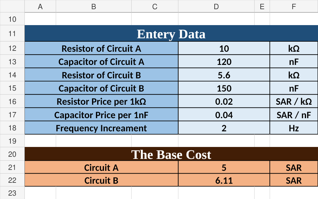
The project compares two passive first-order RC low-pass filter configurations for a hypothetical compact audio application. Circuit A uses 10 kΩ and 120 nF; Circuit B uses 5.6 kΩ and 150 nF. Excel organizes the inputs, calculates ideal magnitude and dB gain, applies frequency-band cost multipliers, and evaluates 251 points from 0 to 500 Hz.

The project remained analytical. It did not include physical circuit construction, SPICE simulation, oscilloscope measurement, listening tests, or integration into an actual Bluetooth speaker.

03Definition

Engineering Problem & Objectives

The design problem was to select between two RC alternatives for an application prioritizing response around 150 Hz while remaining sensitive to modeled component cost.

The comparison was intentionally bounded to ideal first-order equations and assignment-defined economic inputs. Its purpose was a traceable analytical decision, not proof of physical audio performance.

01Define the two component combinations.
02Calculate ideal magnitude response and dB gain.
03Compare both circuits across 0–500 Hz with attention to 150 Hz.
04Include assignment-defined component costs and frequency multipliers.
05Compare gain and cost using a custom project index.
06Make a bounded recommendation without overstating validation.

04Operation

How the Filter Model Works

A first-order RC low-pass filter passes lower frequencies with less attenuation and progressively reduces output magnitude as frequency rises. At cutoff, the ideal magnitude is approximately 0.707, or −3.01 dB.

01Define inputs

02Build sweep

03Find angular frequency

04Calculate magnitude

05Convert to dB

06Weight cost

07Calculate index

08Compare

The workbook generates a 0–500 Hz sweep in 2 Hz increments, then applies the same ideal unloaded equations to Circuit A and Circuit B at every point.

Calculated response, frequency-weighted cost, and the project-defined performance index are compared before making a recommendation within the stated model assumptions.

Seven-step Excel modeling workflow from circuit inputs and frequency sweep through response, weighted cost, performance index, and recommendation. — The analytical workflow applied the same equations and assumptions to both filter configurations.

05Configuration

Circuit Configurations & Parameters

Both alternatives use the same passive first-order topology. Their component values produce different RC time constants, cutoff frequencies, and assignment-defined base costs.

Resistance

Circuit A: 10 kΩ
Circuit B: 5.6 kΩ

Capacitance

Circuit A: 120 nF
Circuit B: 150 nF

RC time constant

Circuit A: 1.20 ms
Circuit B: 0.84 ms

Calculated cutoff

Circuit A: 132.63 Hz
Circuit B: 189.47 Hz

Modeled base cost

Circuit A: 5.000 SAR
Circuit B: 6.112 SAR

Circuit A and Circuit B parameter comparison
Parameter	Circuit A	Circuit B
Resistance	10 kΩ	5.6 kΩ
Capacitance	120 nF	150 nF
RC time constant	1.20 ms	0.84 ms
Calculated cutoff	132.63 Hz	189.47 Hz
Modeled base cost	5.000 SAR	6.112 SAR

Model range: 0–500 Hz in 2 Hz increments, for 251 evaluated points.
Assignment-defined coefficients: 0.02 SAR per kΩ and 0.04 SAR per nF.
Frequency-band multipliers: 1.1, 1.0, 1.2, and 1.3.
The cost inputs are model assumptions, not verified supplier pricing.

Side-by-side ideal RC low-pass circuits: Circuit A uses 10 kΩ and 120 nF; Circuit B uses 5.6 kΩ and 150 nF. — The two alternatives use the same first-order topology but different RC time constants and calculated cutoff frequencies.

06Reasoning

Key Engineering Decisions

Seven bounded decisions define what the workbook compares, why the comparison is useful, and where its conclusions stop.

Decision

Keep the topology constant

Compare the same passive first-order RC low-pass arrangement with two component combinations.

Rationale: Holding topology constant isolates the influence of R and C on calculated cutoff and response.
Trade-off: The study does not compare higher-order, active, or alternative filter topologies.

Decision

Use 150 Hz as the reference point

Anchor the decision around the target selected for the hypothetical compact audio application.

Rationale: A shared reference makes the response and cost comparison concrete.
Trade-off: One simplified target frequency cannot represent complete perceived audio quality.

Decision

Evaluate a 2 Hz frequency sweep

Calculate 251 points from 0 through 500 Hz.

Rationale: The fixed increment provides a traceable view of both response curves around the target.
Trade-off: The resolution adds workbook detail without adding physical validation.

Decision

Use ideal unloaded equations

Model each circuit with the standard first-order transfer function.

Rationale: The same analytical basis keeps the two alternatives directly comparable.
Trade-off: Source impedance, load impedance, tolerances, parasitics, and environmental effects remain outside the model.

Decision

Apply frequency-band cost weighting

Multiply each base cost by the assignment-defined band factor.

Rationale: The workbook requirement introduces an economic dimension alongside calculated response.
Trade-off: The result is a frequency-weighted cost metric, not a changing physical hardware price.

Decision

Use a custom gain-to-cost index

Divide gain in dB by weighted cost to support the workbook comparison.

Rationale: The index combines two assignment criteria in one project-defined academic heuristic.
Trade-off: It is not an industry-standard performance metric and depends on the chosen cost assumptions.

Decision

Keep the recommendation model-bounded

Select Circuit B only within the analytical assumptions.

Rationale: Circuit B retains more calculated response near 150 Hz under the workbook’s comparison method.
Trade-off: The selection does not establish better perceived bass, distortion, or real-world audio performance.

07Model

Mathematical Model

The workbook expresses the ideal first-order response and both project-defined cost measures as accessible, repeatable calculations.

Angular frequency

ω = 2πf

Converts each frequency-sweep value from hertz to radians per second.

Transfer function

H(jω) = 1 / (1 + jωRC)

Represents the ideal unloaded first-order RC low-pass network.

Magnitude

|H(jω)| = 1 / √(1 + (ωRC)²)

Calculates the modeled output-to-input magnitude ratio.

Cutoff frequency

f_c = 1 / (2πRC)

Locates the ideal −3.01 dB point for each component combination.

Gain

G_dB = 20 log₁₀ |H(jω)|

Converts the modeled magnitude ratio to decibels.

Base cost

C_base = R_kΩ(0.02) + C_nF(0.04)

Applies the assignment-defined resistor and capacitor coefficients.

Frequency-weighted cost

C_weighted = C_base × band multiplier

Applies the workbook’s comparison multiplier without implying that physical price changes with frequency.

Performance index

I_project = G_dB / C_weighted

Defines the project’s academic gain-to-cost heuristic; it is not an industry-standard metric.

Magnitude

Circuit A: 0.662
Circuit B: 0.784

Gain

Circuit A: −3.58 dB
Circuit B: −2.11 dB

Project-defined index

Circuit A: −0.716 dB/SAR
Circuit B: −0.346 dB/SAR

Calculated circuit results at 150 hertz
Calculated at 150 Hz	Circuit A	Circuit B
Magnitude	0.662	0.784
Gain	−3.58 dB	−2.11 dB
Project-defined index	−0.716 dB/SAR	−0.346 dB/SAR

At 150 Hz, Circuit B retains approximately 18.4% more modeled output magnitude than Circuit A. This comparison is calculated and is not a measured loudness claim.

The frequency-weighted cost and performance index are assignment-defined comparison tools. Neither should be interpreted as verified supplier pricing or an industry-standard measure of filter quality.

08Implementation

Excel Model Implementation

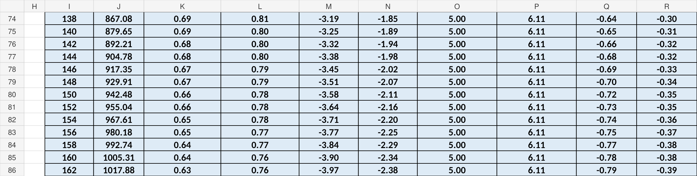
The worksheet connects editable circuit inputs, base-cost calculations, a ten-column 251-row calculation table, frequency-band averages, and charts.

Each row contains frequency, angular frequency, both magnitudes, both dB gains, both weighted costs, and both performance indices. The implementation uses PI(), SQRT(), LOG10(), nested IF(), AVERAGE(), and absolute cell references to propagate the model consistently.

Sanitized Excel input area listing both circuit values, cost coefficients, frequency increment, and calculated base costs. — The workbook centralizes model inputs and base-cost calculations before the frequency sweep.

Sanitized Excel calculation rows from 138 to 162 Hz, including magnitude, gain, weighted cost, and performance index for both circuits. — Calculation rows surrounding the 150 Hz decision point demonstrate how the model propagates the same formulas across the frequency sweep.

Evidence boundary

These sanitized worksheet views document model structure and formula propagation. They do not represent SPICE validation, laboratory measurement, or physical circuit testing.

09Comparison

Comparative Analysis

Circuit A has the lower modeled base cost and lower cutoff, so its calculated response begins attenuating earlier and retains less magnitude at 150 Hz.

Circuit B carries a 22.24% higher modeled base cost, but its higher cutoff retains more calculated response around the target. At 150 Hz, it has 1.46 dB less calculated attenuation and the more favorable project-defined index.

Calculated gain curves from 0 to 500 Hz for Circuit A and Circuit B, marking both cutoff frequencies and the 150 Hz target. — Circuit A attenuates earlier, while Circuit B retains more of the modeled response near 150 Hz. Values are analytical and were not physically measured.

Grouped bars comparing the assignment-defined frequency-weighted cost of Circuit A and Circuit B across four frequency bands. — Circuit A remains the lower-cost alternative across all modeled bands. The values are weighting metrics, not frequency-dependent physical prices.

Project-defined gain-to-weighted-cost performance-index curves for both circuits across 0 to 500 Hz. — Circuit B remains closer to zero around the target region under the workbook’s custom academic heuristic. This is not a standard industry metric.

10Outcome

Results & Recommendation

Within the model assumptions, Circuit B was recommended because its 189.47 Hz cutoff allows more modeled response around 150 Hz.

The recommendation balances the calculated response advantage against the higher assignment-defined base cost; it does not extend beyond the ideal analytical comparison.

Calculated cutoff

Circuit A: 132.63 Hz
Circuit B: 189.47 Hz

Magnitude at 150 Hz

Circuit A: 0.662
Circuit B: 0.784

Gain at 150 Hz

Circuit A: −3.58 dB
Circuit B: −2.11 dB

Modeled base cost

Circuit A: 5.000 SAR
Circuit B: 6.112 SAR

Project-defined index at 150 Hz

Circuit A: −0.716
Circuit B: −0.346

Selection within model assumptions

Circuit A: —
Circuit B: Recommended

Circuit comparison and recommendation
Metric	Circuit A	Circuit B
Calculated cutoff	132.63 Hz	189.47 Hz
Magnitude at 150 Hz	0.662	0.784
Gain at 150 Hz	−3.58 dB	−2.11 dB
Modeled base cost	5.000 SAR	6.112 SAR
Project-defined index at 150 Hz	−0.716	−0.346
Selection within model assumptions	—	Recommended

Circuit B retains more modeled response at the target frequency, while carrying the higher assignment-defined base cost.

Boundary: the recommendation does not prove better perceived bass, lower distortion, or superior real-world audio performance.

11Reflection

Limitations & Takeaways

The comparison is useful only when its ideal assumptions, academic cost model, and unvalidated physical behavior remain explicit.

Model limitations

Ideal component values.
No source or load impedance.
No parasitic or environmental effects.
No SPICE validation.
No physical circuit or measurements.
No listening or speaker testing.
One simplified target frequency.
Assignment-defined cost coefficients.
A nonstandard custom performance index.

Engineering takeaways

Simple circuits can still involve meaningful trade-offs.
“Better” depends on the requirement.
Models support but do not replace validation.
Economic assumptions influence recommendations.
Traceable calculations improve decision-making.
Calculated, simulated, measured, and observed are not interchangeable.

12Next steps

Future Direction & Resources

Future work would replace ideal assumptions with circuit, tolerance, physical, and economic validation before making a real product decision.

Future direction

Include source and load impedance.
Evaluate component tolerances and Monte Carlo variation.
Validate both configurations in SPICE.
Construct and measure the circuits.
Test with a representative amplifier, loudspeaker, and enclosure.
Compare higher-order and active filter options.
Replace model coefficients with supplier and production data.
Replace the custom index with a clearer multi-criteria decision method.